21. Tuning Strategies 2

Gradient Descent Algorithm ("Twiddle")

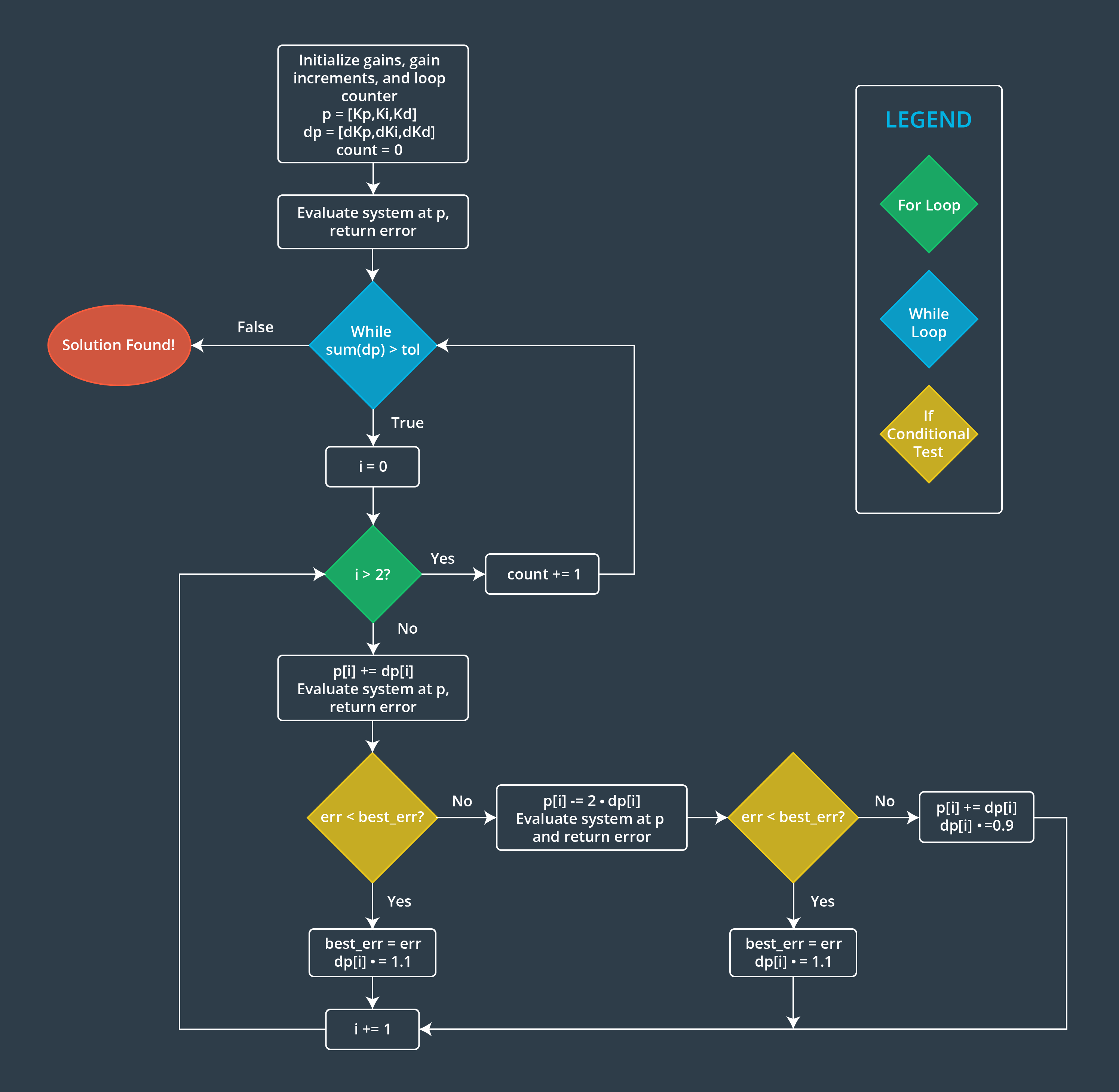
A more automatic approach is to use a gradient descent algorithm, sometimes referred to as “Twiddle”. The premise is that you start with a vector of initial guesses for the three gains. A small non-zero value for P, and zeros for I and D is generally recommended. Then you individually make small changes to each of the gains and test if the cost function decreases. If it does, you keep changing the parameter in the same direction, otherwise you try adjusting the parameter in the opposite direction. If neither an increase or a decrease in the gain value decreases the cost function then you reduce the size of the gain increment and repeat. The whole cycle should continue until the size of the increment falls below some threshold value.

One of the challenges is to decide what the error function should be: maximum percent overshoot? Settling time? Some linear combination of them? Ultimately the error function must be distilled into a single scalar value that has a clear magnitude.

Start Quiz:

#!/usr/bin/env python
import numpy as np
import matplotlib.pyplot as plt

'''Your job is to complete the twiddle function. I have written a
   cost function for your that attempts to minimize percent overshoot.
   Feel free to modify the cost function! Just remember that the cost
   function must return a single scalar value.
'''

def ydot(y, t, dt, r, p):
    ''' ydot returns the next state of the quadrotor as a function of
    the current state and control inputs.
    Parameters:
    -----------
    y = augmented state vector (7 element list)
    t = time, (sec)
    dt = time-step, (sec)
    r = controller setpoint, (m)
    p = list of PID gains = [kp, ki, kd]
    '''
    # Model states
    y1 = y[0] # altitude, (m)
    y2 = y[1] # speed, (m/s)
    y3 = y[2] # last error, (m)
    y4 = y[3] # integral of error, (m*sec)
    y5 = y[4] # proportional effort term, (m/s/s)
    y6 = y[5] # integral effort term, (m/s/s)
    y7 = y[6] # derivative effort term, (m/s/s)

    # Current position error, (m)
    e = r - y1

    # Control Effort (i.e., net motor thrust)
    Kp = p[0]
    Ki = p[1]
    Kd = p[2]
    up = Kp*e # proportional control effort
    ui = Ki*(e*dt + y4) # integral control effort
    ud = Kd*(e - y3)/dt # derivative control effort
    u = up + ui + ud # total control effort

    # Actuator limits
    if u > umax:
        u = umax # max possible output
    elif u < 0:
        u = 0 # the quadrotor's motors cannot run in reverse

    ### State derivatives
    # if altitude = 0
    if (y1 <= 0.):
    # if control input, u <= gravity, vehicle stays at rest on the ground
    # this prevents quadrotor from "falling" through the ground if thrust is
    # too small.
        if u <= np.absolute(g*m/c):
            y1dot = 0.
            y2dot = 0.
        else:
            # if u > gravity and quadrotor accelerates upwards
            y1dot = y2
            y2dot = g + c/m*u - 0.75*y2
    else: # otherwise quadrotor is already in the air
        y1dot = y2
        y2dot = g + c/m*u - 0.75*y2

    # Calculate new state
    y1 += y1dot*dt
    y2 += y2dot*dt
    y3 = e
    y4 += e*dt
    y5 = up
    y6 = ui
    y7 = ud
    return [y1, y2, y3, y4, y5, y6, y7]

def hover(p):
    ''' This function simulates the quadrotor's
        motion in response to a step change in the altitude setpoint.
        The states as a function of time are stored in the np.array, soln.
    '''
    # Inital conditions
    y = [0, 0, 0, 0, 0, 0, 0]
        #y[0] = initial altitude, (m)
        #y[1] = initial speed, (m/s)
        #y[2] = current error, (m)
        #y[3] = integral of error, (m*sec)
        #y[4] = proportional control
        #y[5] = integral control
        #y[6] = derivative control
    # Initialize array to store values
    soln = np.zeros((len(time),len(y)))

    j = 0 # dummy counter
    for t in time:
        y = ydot(y,t,dt,r,p)
        soln[j,:] = y
        j += 1
    return soln

def cost_fun(soln):
    '''
    This is the function that Twiddle is trying to optimize.
    FEEL FREE TO WRITE YOUR OWN COST-FUNCTION!!!
    Here I have it trying to minimize overshoot.
    '''
    y0 = soln[:,0] #altitude
    rise_time_index =  np.argmax(y0>r)
    RT = time[rise_time_index]

    OS = (np.max(y0) - r)/r*100
    OS_pen = OS
    if OS < 0:
        OS = 0
        OS_pen = 100
    #return OS_pen**2 + RT**2
    return OS_pen**2

def twiddle(tol=0.05):
    # initial gain estimates
    p = [2, 2, 2]
    dp = [0.10, 0.10, 0.10]
    #robot = make_robot()
    #x_trajectory, y_trajectory, best_err = run(robot, p)
    soln = hover(p)
    best_cost = cost_fun(soln)

    # TODO: Complete the Twiddle ALgorithm
    #
    #
    #######################################
    return p
    

# Simulation parameters
N = 500 # number of simultion points
t0 = 0  # starting time, (sec)
tf = 30 # end time, (sec)
time = np.linspace(t0, tf, N)
dt = time[1] - time[0] # delta t, (sec)
r = 10 # altitude setpoint, (m)

# Model parameters
g = -9.81 # gravity, m/s/s
m =  1.54 # quadrotor mass, kg
c = 10.   # electro-mechanical transmission constant
umax = 5.0 # max controller output, (m/s/s)

p = twiddle()
print(p)
soln = hover(p)

# Plot results
SP = np.ones_like(time)*r # altitude set point
UMAX = np.ones_like(time)*umax
fig = plt.figure()
ax1 = fig.add_subplot(311)
ax1.plot(time, soln[:,0],time,SP,'--')
ax1.set_xlabel('Time, (sec)')
ax1.set_ylabel('Altitude, (m)')
ax2 = fig.add_subplot(312)
ax2.plot(time, soln[:,1])
ax2.set_xlabel('Time, (sec)')
ax2.set_ylabel('Speed, (m/s)')

ax3 = fig.add_subplot(313)
ax3.plot(time, soln[:,4], '-r', label="Up")
ax3.plot(time, soln[:,5], '-b', label="Ui")
ax3.plot(time, UMAX,'--k', label="Umax")
ax3.set_xlabel('Time, (sec)')
ax3.set_ylabel('Cont. Effort, (m/s/s)')
ax3.legend(loc='upper left')
plt.tight_layout()
plt.show()
#!/usr/bin/env python
import numpy as np
import matplotlib.pyplot as plt

'''Your job is to complete the twiddle function. I have written a
   cost function for your that attempts to minimize percent overshoot.
   Feel free to modify the cost function! Just remember that the cost
   function must return a single scalar value.
'''

def ydot(y, t, dt, r, p):
    ''' ydot returns the next state of the quadrotor as a function of
    the current state and control inputs.
    Parameters:
    -----------
    y = augmented state vector (7 element list)
    t = time, (sec)
    dt = time-step, (sec)
    r = controller setpoint, (m)
    p = list of PID gains = [kp, ki, kd]
    '''
    # Model states
    y1 = y[0] # altitude, (m)
    y2 = y[1] # speed, (m/s)
    y3 = y[2] # last error, (m)
    y4 = y[3] # integral of error, (m*sec)
    y5 = y[4] # proportional effort term, (m/s/s)
    y6 = y[5] # integral effort term, (m/s/s)
    y7 = y[6] # derivative effort term, (m/s/s)

    # Current position error, (m)
    e = r - y1

    # Control Effort (i.e., net motor thrust)
    Kp = p[0]
    Ki = p[1]
    Kd = p[2]
    up = Kp*e # proportional control effort
    ui = Ki*(e*dt + y4) # integral control effort
    ud = Kd*(e - y3)/dt # derivative control effort
    u = up + ui + ud # total control effort

    # Actuator limits
    if u > umax:
        u = umax # max possible output
    elif u < 0:
        u = 0 # the quadrotor's motors cannot run in reverse

    ### State derivatives
    # if altitude = 0
    if (y1 <= 0.):
    # if control input, u <= gravity, vehicle stays at rest on the ground
    # this prevents quadrotor from "falling" through the ground if thrust is
    # too small.
        if u <= np.absolute(g*m/c):
            y1dot = 0.
            y2dot = 0.
        else:
            # if u > gravity and quadrotor accelerates upwards
            y1dot = y2
            y2dot = g + c/m*u - 0.75*y2 #NOTE: I added damping to make the system easier to control
    else: # otherwise quadrotor is already in the air
        y1dot = y2
        y2dot = g + c/m*u - 0.75*y2 #NOTE: I added damping to make the system easier to control

    # Calculate new state
    y1 += y1dot*dt
    y2 += y2dot*dt
    y3 = e
    y4 += e*dt
    y5 = up
    y6 = ui
    y7 = ud
    return [y1, y2, y3, y4, y5, y6, y7]

def hover(p):
    ''' This function simulates the quadrotor's
        motion in response to a step change in the altitude setpoint.
        The states as a function of time are stored in the np.array, soln.
    '''
    # Inital conditions
    y = [0, 0, 0, 0, 0, 0, 0]
        #y[0] = initial altitude, (m)
        #y[1] = initial speed, (m/s)
        #y[2] = current error, (m)
        #y[3] = integral of error, (m*sec)
        #y[4] = proportional control
        #y[5] = integral control
        #y[6] = derivative control
    # Initialize array to store values
    soln = np.zeros((len(time),len(y)))

    j = 0 # dummy counter
    for t in time:
        y = ydot(y,t,dt,r,p)
        soln[j,:] = y
        j += 1
    return soln

def cost_fun(soln):
    '''
    This is the function that Twiddle is trying to optimize.
    FEEL FREE TO WRITE YOUR OWN COST-FUNCTION!!!
    Here I have it trying to minimize overshoot.
    '''
    y0 = soln[:,0] #altitude
    rise_time_index =  np.argmax(y0>r)
    RT = time[rise_time_index]

    OS = (np.max(y0) - r)/r*100
    OS_pen = OS
    if OS < 0:
        OS = 0
        OS_pen = 100
    #return OS_pen**2 + RT**2
    return OS_pen**2

def twiddle(tol=0.05):
    p = [2, 2, 2]
    dp = [0.10, 0.10, 0.10]
    soln = hover(p)
    best_cost = cost_fun(soln)

    ### TO DO: Complete the Twiddle ALgorithm
    it = 0
    while sum(dp) > tol:
        print("Iteration {}, best error = {}".format(it, best_cost))
        for i in range(len(p)):
            p[i] += dp[i]
            # Can't have negative gains
            if p[i] < 0:
                p[i] = 0
            soln = hover(p)
            cost = cost_fun(soln)

            if cost < best_cost:
                best_cost = cost
                dp[i] *= 1.1
            else:
                p[i] -= 2 * dp[i]
                # Can't have negative gains
                if p[i] < 0:
                    p[i] = 0
                soln = hover(p)
                cost = cost_fun(soln)

                if cost < best_cost:
                    best_cost = cost
                    dp[i] *= 1.1
                else:
                    p[i] += dp[i]
                    # Can't have negative gains
                    if p[i] < 0:
                        p[i] = 0
                    dp[i] *= 0.9
        it += 1
    return p


# Simulation parameters
N = 500 # number of simultion points
t0 = 0  # starting time, (sec)
tf = 30 # end time, (sec)
time = np.linspace(t0, tf, N)
dt = time[1] - time[0] # delta t, (sec)
r = 10 # altitude setpoint, (m)

# Model parameters
g = -9.81 # gravity, m/s/s
m =  1.54 # quadrotor mass, kg
c = 10.   # electro-mechanical transmission constant
umax = 5.0 # max controller output, (m/s/s)

p = twiddle()
print(p)
soln = hover(p)

# Plot results
SP = np.ones_like(time)*r # altitude set point
UMAX = np.ones_like(time)*umax
fig = plt.figure()
ax1 = fig.add_subplot(311)
ax1.plot(time, soln[:,0],time,SP,'--')
ax1.set_xlabel('Time, (sec)')
ax1.set_ylabel('Altitude, (m)')
ax2 = fig.add_subplot(312)
ax2.plot(time, soln[:,1])
ax2.set_xlabel('Time, (sec)')
ax2.set_ylabel('Speed, (m/s)')

ax3 = fig.add_subplot(313)
ax3.plot(time, soln[:,4], '-r', label="Up")
ax3.plot(time, soln[:,5], '-b', label="Ui")
ax3.plot(time, UMAX,'--k', label="Umax")
ax3.set_xlabel('Time, (sec)')
ax3.set_ylabel('Cont. Effort, (m/s/s)')
ax3.legend(loc='upper left')
plt.tight_layout()
plt.show()